Serving, Capacity & Load Testing: Math → Code

How to size, configure, benchmark, and explain an LLM deployment, organized as math first, then the code and engine flags that implement it. Written for the engineer who inherits a customer deployment from an ML or performance engineer at an inference cloud and must defend every number to both a researcher and a buyer. Engine flags reviewed against the vLLM and SGLang docs in October 2026.

Parent topic: LLM Systems & Inference. Runnable, stdlib-only tools live in code/: a capacity calculator and an open-loop load generator with an offline mock engine.

Overview

Primary references (all free): PagedAttention / vLLM (2309.06180), Orca (OSDI 2022, iteration-level scheduling), Sarathi-Serve (2403.02310), DistServe (2401.09670), Splitwise (2311.18677), Mooncake (2407.00079), vLLM docs (free), SGLang docs (free)
Supplementary (free): How to Scale Your Model (rooflines, inference chapter), Making Deep Learning Go Brrrr, Databricks’ LLM Inference Performance Engineering (MBU), speculative decoding (2211.17192), Medusa (2401.10774), EAGLE-3 (2503.01840), Punica (2310.18547), S-LoRA (2311.03285), SGLang / RadixAttention (2312.07104), NVIDIA Dynamo, TensorRT-LLM
Prerequisites: LLM Systems & Inference (prefill, decode, KV cache), Quantization (what FP8/INT4 buys), Probability & Statistics (Poisson, percentiles), Observability
Estimated time: 2-3 weeks at 8-10 hrs/week

Key Takeaways

Decode is a bandwidth problem, prefill is a compute problem. A decode step reads every weight once to produce one token per sequence, so tok/s per sequence ≤ HBM bandwidth / bytes per step. Batching amortizes that read, which is the whole economic engine of an inference cloud
Memory decides concurrency. After weights, every remaining byte is KV cache, and KV/token = 2 × layers × kv_heads × head_dim × bytes. Concurrency, context length, and cost per token all fall out of that one division
SLOs are distributions. TTFT and TPOT at p99 under a stated arrival process are the contract; mean throughput at infinite load is a marketing number. Report goodput: requests per second that meet every SLO
Every knob moves a point along one curve. Bigger batches raise throughput and raise TPOT; chunked prefill trades a little TTFT for stable TPOT; speculative decoding buys latency at low load and costs throughput at high load
Benchmark open loop with realistic lengths, a warmup, and no accidental prefix-cache hits, then show the customer the latency-throughput curve and the cost per 1M tokens at their SLO point

How to Study

Run code/capacity.py for the model your customer asked about before reading anything else, then derive each printed line by hand
Run code/loadgen.py --mock --sweep and watch TTFT p99 explode once offered load passes capacity; then repeat against a real vllm serve on one GPU
For each engine flag, write down which term of the memory budget or the step-time equation it changes. If you cannot, you do not yet understand the flag
Read Orca, then PagedAttention, then Sarathi-Serve, then DistServe in that order: each fixes the bottleneck the previous one exposed

Concepts & Techniques

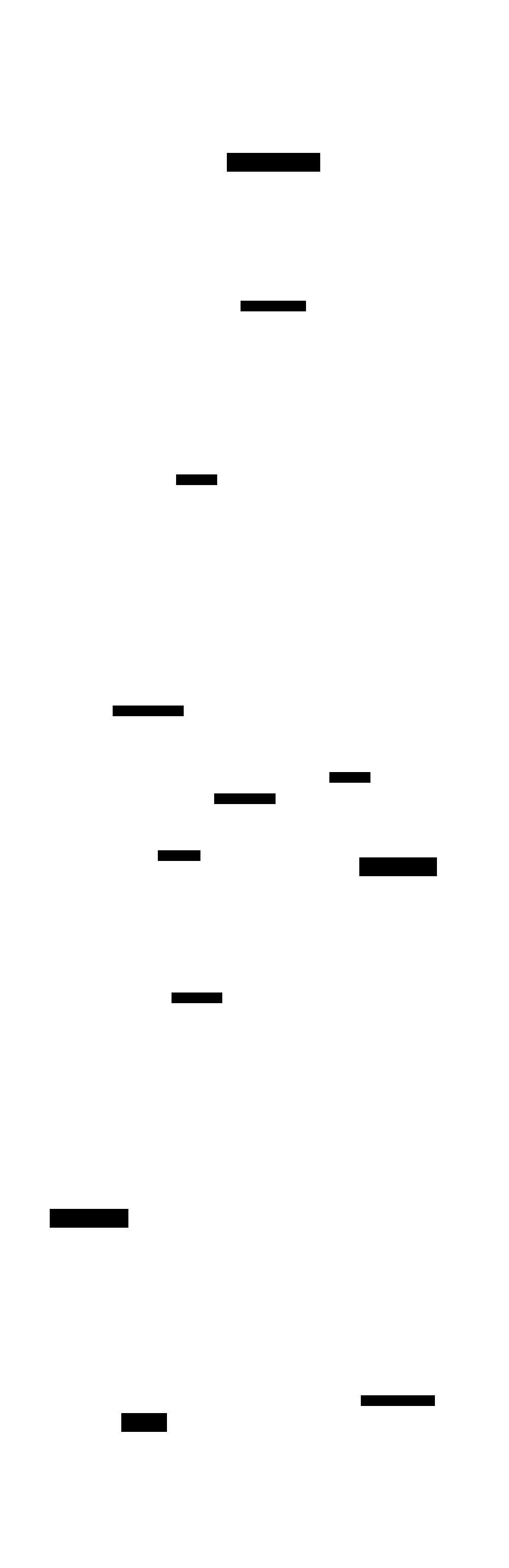
Core Insight

A serving engine runs a loop: pick a batch of sequences, run one forward pass, append one token to each (or a chunk of prompt for prefilling ones), repeat. The step time of that loop is

t_step ≈ max( FLOPs_step / (peak_FLOPs × MFU),  bytes_step / (HBM_BW × MBU) ) + t_comm + t_overhead
bytes_step ≈ W_active / N_gpu + Σ_seq ctx_seq × KV_tok / N_gpu

Every metric a customer cares about is a function of that equation: TPOT is t_step during decode, TTFT is queueing plus the prefill steps, throughput is batch / t_step, and cost is $/hr / throughput. Every engine knob changes a term of it (batch size, bytes per weight, bytes per KV element, N_gpu, how prefill tokens are mixed in). The FDE’s job is to know which term dominates for this customer’s traffic and move that one.

Where that loop sits in a production stack: the gateway and router decide which replica runs a request; the engine’s scheduler and KV cache manager decide when and with how much memory; the autoscaler closes the loop on queue depth and KV utilization.

LLM serving stack: client, gateway, router, engine replicas with scheduler, KV cache manager and executor, GPUs, autoscaler, and weight storage

1. Prefill vs Decode: The Roofline

Key ideas:

Arithmetic intensity I = FLOPs / bytes moved. The roofline says attainable throughput is min(peak_FLOPs, I × BW). The ridge point I* = peak / BW separates memory-bound (I < I*) from compute-bound
H100 SXM: 989 TFLOP/s dense BF16, 1979 dense FP8, 3.35 TB/s HBM3. So I* ≈ 295 FLOP/B for BF16 and ≈ 590 FLOP/B for FP8. H200 keeps the FLOPs and raises bandwidth to 4.8 TB/s, which is why it decodes faster at the same price class
Linear layers dominate FLOPs: for a d_in × d_out weight and T tokens in the step, FLOPs = 2 T d_in d_out, weight bytes = b d_in d_out, so I ≈ 2T / b. At BF16 (b = 2), intensity equals the number of tokens in the step
Prefill: T = prompt length (e.g. 2048), so I ≈ 2048 ≫ 295. Compute-bound. Lower bound on prefill time: t ≈ 2 P n / (peak × MFU). Llama-3.1-8B, 2048 tokens: 2 × 8e9 × 2048 / 989e12 ≈ 33 ms at 100% MFU, roughly 50-60 ms in practice
Decode: T = batch size B (one new token per sequence). At B = 1, I ≈ 1: the GPU is about 300x underused on compute. The step costs one full read of the weights plus the KV history
Decode bound: tok/s per sequence ≤ BW × MBU / (W/N + ctx × KV_tok / N). Llama-3.1-8B BF16 on one H100: 3.35e12 / 16.06e9 ≈ 209 tok/s from weights alone, about 202 with a 4k-token KV history. Real engines reach MBU of 60-85%
Batch effect: increasing B adds only KV bytes per step (weights are shared), so aggregate tok/s rises almost linearly until either (a) the KV reads dominate, (b) KV memory runs out, or (c) B approaches I* and decode turns compute-bound. Attention itself never batches: each sequence reads its own KV, intensity about 1 (GQA raises it to the group size)
MoE: per-token FLOPs scale with active params, but at large batch nearly every expert is touched each step, so bytes per step trend toward total params. MoE is cheap at high batch and expensive at batch 1

Math → code: the decode section of capacity.py.

w_read = m.active * a.weight_bytes / n_gpus              # weights touched per step, per GPU
step_bytes_b = w_read + batch * avg_ctx * kv_tok_per_gpu  # plus every sequence's KV history
t_mem_b = step_bytes_b / (hbm_bw * mbu)
t_cmp_b = 2 * m.active * batch / (peak * tp)              # linear-layer FLOPs
agg_tok_s = batch / max(t_mem_b, t_cmp_b)

2. The Memory Budget

Key ideas:

Weights: W = params × bytes/param. BF16 = 2, FP8/INT8 = 1, INT4 ≈ 0.5 plus group scales. Sharded W/TP per GPU under tensor parallelism
KV cache per token: KV_tok = 2 × L × n_kv × d_head × b_kv. The 2 is K and V. Sharded across TP ranks by KV head, but replicated once TP > n_kv
GQA shrinks n_kv: Llama-3.1-8B has 32 query heads but 8 KV heads, so 128 KiB/token instead of 512 KiB under MHA. That 4x is 4x the concurrent users
MLA (DeepSeek-V2/V3) caches one compressed latent per layer shared by all heads: KV_tok = L × (d_c + d_rope) × b = 61 × (512 + 64) × b. At FP8 that is 34.3 KiB/token for a 671B model, smaller than the 8B Llama at BF16. The latent is replicated across TP ranks, which is why DeepSeek deployments use DP attention (SGLang --enable-dp-attention) or decode context parallelism (vLLM --decode-context-parallel-size)
Activation headroom: the engine profiles a forward pass at max_num_batched_tokens at startup, plus CUDA graph pools and NCCL buffers. Budget 1-4 GiB per GPU; more for large vocabularies (the logits tensor is tokens × vocab × 4 B)
Budget: KV_pool = util × M_gpu − W/N − activations. vLLM’s --gpu-memory-utilization and SGLang’s --mem-fraction-static set util
Concurrency: max_tokens = KV_pool / KV_tok_per_gpu; max_seqs = max_tokens / ctx. With PagedAttention the context that counts is the live one, not max_model_len: requests only hold the blocks they have filled

Worked example: H100 80 GiB, util = 0.90, 2 GiB reserve, 8,192-token sequences. Output of capacity.py:

Config	GPUs	Weights/GPU	KV pool/GPU	KV/token/GPU	Max KV tokens	Seqs @ 8k	Single-stream bound
8B BF16, BF16 KV	1	14.96 GiB	55.04 GiB	128 KiB	450,912	55	202 tok/s
8B FP8, FP8 KV	1	7.48 GiB	62.52 GiB	64 KiB	1,024,352	125	404 tok/s
70B BF16	1	131.5 GiB	does not fit
70B BF16, TP=2	2	65.75 GiB	4.25 GiB	160 KiB	27,844	3.4	47 tok/s
70B BF16, TP=4	4	32.88 GiB	37.12 GiB	80 KiB	486,596	59	94 tok/s
70B FP8, FP8 KV	1	65.75 GiB	4.25 GiB	160 KiB	27,844	3.4	47 tok/s
70B FP8, FP8 KV, TP=2	2	32.88 GiB	37.12 GiB	80 KiB	486,596	59	94 tok/s

Read the table the way a customer will: 70B BF16 on 2 GPUs technically fits and is useless (3 concurrent 8k sequences). FP8 on TP=2 gives the same concurrency as BF16 on TP=4 at half the GPUs, which is why FP8 (with an accuracy check, see Quantization) is the default recommendation for 70B-class dense models on Hopper.

python code/capacity.py --preset llama-3.1-70b --tp 2 --weight-bytes 1 --kv-bytes 1

3. Metrics, SLOs, and Little’s Law

Key ideas:

TTFT (time to first token): queueing + prefill (+ network). Governs perceived responsiveness for chat and streaming UIs
TPOT (time per output token) = (E2E − TTFT) / (n_out − 1), a per-request average. ITL (inter-token latency) is each individual gap; its p99 exposes stalls that the TPOT average hides (a long prefill scheduled into the batch freezes every decoding stream for one step)
E2E latency ≈ TTFT + TPOT × (n_out − 1). What batch and agent workloads care about
Throughput: output tok/s (decode capacity), total tok/s (input + output, for prefill-heavy RAG), req/s. Always say which
Goodput (DistServe): the max request rate at which at least X% of requests meet both the TTFT and TPOT SLOs. It is the number that sets the price
Percentiles: p50 for typical experience, p99 for the contract. p99 of a mean is meaningless; compute percentiles over requests (or over individual ITL gaps), never over per-second averages
The latency-throughput curve: plot TPOT p50/p99 and TTFT p99 against achieved throughput as offered load rises. TPOT rises slowly (bigger batches), then TTFT goes vertical when arrival rate exceeds service rate and the queue grows without bound. The usable operating point is the knee, before the vertical
Little’s law: L = λ × W. Mean in-flight requests equals arrival rate times mean time in system. At 10 req/s and 6 s mean E2E, 60 requests are in flight: you need --max-num-seqs ≥ 60 and a KV pool for 60 × mean context tokens, or the excess queues and TTFT grows
Utilization and queueing: for an M/M/1-like server, mean wait grows as ρ / (1 − ρ). At 90% utilization the queue is 9x the service time; at 95% it is 19x. Size for 60-75% of measured saturation on bursty traffic

One streaming request, end to end. TTFT spans arrival to the first SSE chunk; every later gap is one ITL sample; TPOT is their mean.

sequenceDiagram
    participant C as Client
    participant G as Gateway
    participant S as Scheduler
    participant E as Engine
    participant GPU as GPU
    C->>G: POST /v1/chat/completions (stream true)
    G->>G: auth, rate limit, tokenize prompt
    G->>S: enqueue request (n_in tokens)
    Note over S: waits in queue until KV blocks and batch slot are free
    S->>E: allocate KV blocks, schedule prefill chunk 1
    E->>GPU: forward pass (chunk 1 mixed with running decodes)
    S->>E: schedule prefill chunk 2 (last)
    E->>GPU: forward pass, sample token 1
    E->>G: token 1
    G->>C: SSE chunk 1 (TTFT ends here)
    loop each decode step (one ITL gap per token)
        S->>E: include sequence in batch, grow KV by one slot
        E->>GPU: forward pass for whole batch
        E->>G: token k
        G->>G: incremental detokenize
        G->>C: SSE chunk k
    end
    E->>S: EOS or max_tokens reached
    S->>S: free KV blocks (shared prefix blocks decrement refcount)
    G->>C: final chunk with usage, then [DONE]

Workload	Primary SLO	Typical targets (illustrative)	What to optimize
Chat UI	TTFT p99, TPOT p50	TTFT < 500 ms, TPOT < 30-50 ms (faster than reading)	Prefix caching, chunked prefill, moderate batch
Code completion	TTFT p99, E2E	TTFT < 200 ms, short outputs	Small model, spec decoding, low batch
RAG / long-context QA	TTFT at long inputs	TTFT < 2 s at 32k input	Prefill throughput, prefix cache, disaggregation
Agents / tool loops	E2E per turn	Many sequential calls, each adds TTFT	Prefix caching across turns, spec decoding
Offline batch	Cost per 1M tokens	Throughput only	Max batch, FP8, `--max-num-seqs` high

4. Parallelism: TP, PP, DP, EP, CP, and Disaggregation

Key ideas:

Tensor parallelism (TP) (Megatron-LM): split each matmul across N GPUs. Weights and KV per GPU shrink by N, so per-token latency drops. Cost: 2 all-reduces per layer of T × d × b bytes, ring time ≈ 2(N−1)/N × size / link_BW. Needs NVLink: H100 NVLink 4 gives 900 GB/s per GPU versus about 64 GB/s per direction for PCIe Gen5 x16. Keep TP inside one NVLink domain (8 GPUs on HGX, 72 on GB200 NVL72)
Pipeline parallelism (PP): split layers into stages. One point-to-point send per stage boundary per microbatch, so it tolerates PCIe and InfiniBand (NDR: 400 Gb/s ≈ 50 GB/s per port). Does not reduce single-request latency and adds bubbles; use it to span nodes when a model will not fit in one NVLink domain
Data parallelism (DP): independent replicas behind a load balancer. Throughput scales linearly, latency unchanged, no communication. The default for anything that fits on one GPU or one TP group: two TP=1 replicas of an 8B model beat one TP=2 replica on throughput per GPU
Expert parallelism (EP): for MoE, place whole experts on different GPUs and route tokens with all-to-all. Avoids TP’s per-expert matmul slicing (small experts slice badly). Usually combined with DP attention: attention runs data-parallel, MoE layers run expert-parallel. vLLM --enable-expert-parallel with --data-parallel-size; SGLang --ep-size with --enable-dp-attention
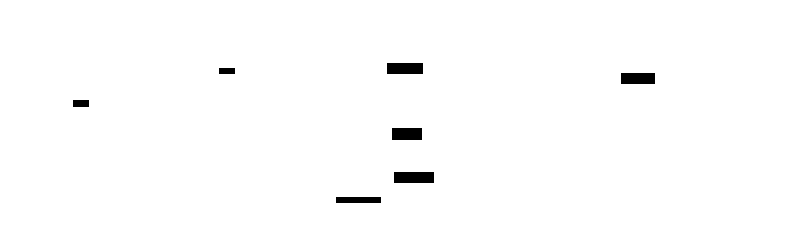
Context / sequence parallelism (CP): split one long sequence’s tokens across GPUs (ring attention style) for prefill of 128k+ prompts, or shard its KV for decode. vLLM exposes --prefill-context-parallel-size and --decode-context-parallel-size
Disaggregated prefill/decode: run prefill and decode on separate GPU pools and ship the KV cache between them. Rationale (DistServe, Splitwise): the phases interfere (a prefill stalls every decode in the batch) and want different parallelism and even different hardware. Mooncake (Kimi) adds a KV-cache-centric store across DRAM/SSD so prefixes are computed once cluster-wide
KV transfer cost decides whether disaggregation pays: shipping n × KV_tok bytes must take less than the decode interference it removes. 8k tokens of 70B BF16 KV is 8192 × 320 KiB ≈ 2.7 GB: about 54 ms at 50 GB/s RDMA, which is why this needs RDMA (NIXL, Mooncake transfer engine) and not TCP
Implementations: vLLM --kv-transfer-config with connectors (NIXL, LMCache, Mooncake); SGLang --disaggregation-mode prefill|decode; NVIDIA Dynamo orchestrates disaggregated vLLM, SGLang, or TensorRT-LLM workers with a KV-aware router and a planner that rebalances prefill vs decode GPUs

How each strategy places the model, and the collective it pays:

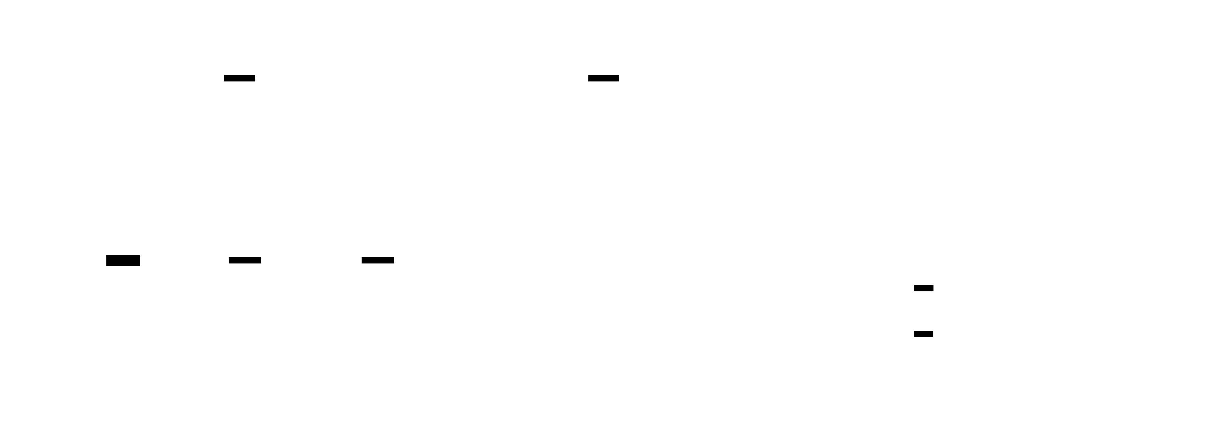
Tensor, pipeline, expert, and data parallelism layouts with their communication

Disaggregated serving moves the prefill/decode split from inside one engine’s batch to two GPU pools, with the router choosing a worker in each and the KV cache crossing RDMA:

Disaggregated prefill and decode pools with KV transfer over NIXL / RDMA

Strategy	Reduces latency	Raises throughput	Interconnect need	Use when
DP	No	Yes, linear	None	Model fits one GPU or one TP group
TP	Yes	Per replica	NVLink	Model too big for one GPU, or TPOT SLO too tight
PP	No	Yes, with bubbles	PCIe / IB fine	Model too big for one node
EP (+ DP attn)	Somewhat	Yes for MoE	NVLink / fast IB all-to-all	Large MoE (DeepSeek, Qwen-MoE, Llama-4)
CP	Yes for long prefill	No	NVLink	128k+ contexts
P/D disaggregation	Stabilizes TPOT and TTFT	Yes at scale	RDMA	Long prompts, strict TPOT, many replicas

Worked TP communication cost (Llama-3.1-70B decode, batch 64, BF16, TP=4 on NVLink):

per all-reduce:   T × d × b = 64 × 8192 × 2 B          = 1.05 MB
ring traffic:     2(N−1)/N × 1.05 MB = 1.5 × 1.05 MB   = 1.57 MB per GPU
per layer:        2 all-reduces                        = 3.1 MB
per step:         80 layers                            = 252 MB
time at ~450 GB/s effective NVLink (one direction)     ≈ 0.56 ms
time at ~50 GB/s effective PCIe Gen5                   ≈ 5 ms

Against a memory-bound step of roughly 16 ms (see capacity.py --preset llama-3.1-70b --tp 4), NVLink adds about 3%; PCIe adds about 30%, before latency effects of 160 small collectives. This is why TP across PCIe-only cards (L40S boxes) is usually capped at 2, and why replicas (DP) beat TP there.

5. Engine Knobs

Key ideas:

Continuous batching (Orca): schedule per iteration, not per request; sequences join and leave the batch every step. Every modern engine does this
PagedAttention (2309.06180): KV in fixed-size blocks with a block table, so memory is allocated as tokens arrive. Removes fragmentation and enables block sharing for prefixes
Chunked prefill (Sarathi-Serve): cap tokens per step (max_num_batched_tokens); long prompts are split into chunks and co-scheduled with decodes. Bounds the step time, so ITL p99 stays flat. Smaller budget: better ITL, worse TTFT for long prompts. Larger: the reverse
Prefix caching: hash KV blocks by token content (vLLM) or keep a radix tree of prefixes (SGLang RadixAttention). System prompts, few-shot examples, multi-turn chat, and agent loops get TTFT near zero for the cached part. SGLang --schedule-policy lpm (longest prefix match) orders the queue to maximize hits
Preemption: when the KV pool fills mid-generation, the engine evicts a sequence and recomputes it later. Visible as TPOT spikes and a preemption counter in metrics. Fix with more KV memory, lower --max-num-seqs, or FP8 KV

vLLM (vllm serve, engine args):

Flag	Term it changes	Notes
`--tensor-parallel-size` / `-tp`	`N` in `W/N`, `KV/N`	Within NVLink domain
`--pipeline-parallel-size` / `-pp`	Layers per GPU	Across nodes
`--data-parallel-size` / `-dp`	Replicas	Also used for DP attention with EP
`--enable-expert-parallel` / `-ep`	MoE layout	EP instead of TP for MoE layers
`--max-model-len`	Max context	Must fit one sequence in the KV pool; lower it to start on small GPUs
`--gpu-memory-utilization`	`util`	Fraction of GPU memory for the engine; the KV pool is what is left after weights and profiling
`--max-num-seqs`	Max batch `B`	Upper bound on concurrency per step
`--max-num-batched-tokens`	Tokens per step	The chunked-prefill budget; defaults vary by version and GPU, read it from the startup log
`--enable-chunked-prefill`	Prefill mixing	On by default in the V1 engine
`--enable-prefix-caching`	Prefix reuse	On by default in V1; `--no-enable-prefix-caching` for clean benchmarks
`--kv-cache-dtype`	`b_kv`	`auto`, `fp8` (and `fp8_e4m3` / `fp8_e5m2` variants)
`--quantization` / `-q`	`b` for weights	`fp8`, `awq`, `gptq`, `compressed-tensors` checkpoints auto-detected
`--speculative-config` / `-sc`	Tokens per step	JSON: `{"method": "eagle3", "model": ..., "num_speculative_tokens": 3}`; methods include `draft_model`, `ngram`, `eagle`, `eagle3`, `mtp`, `suffix`
`--enable-lora`, `--max-loras`, `--max-lora-rank`	Adapter slots	`--max-loras` adapters per batch (default 1), rank options up to 512
`--kv-transfer-config`	P/D disaggregation	JSON naming a KV connector
`--async-scheduling`	CPU overhead	Overlaps scheduling with GPU execution

SGLang (python -m sglang.launch_server, server arguments):

SGLang flag	vLLM analogue	Notes
`--tp-size` / `--tp`	`--tensor-parallel-size`
`--dp-size`	`--data-parallel-size`	Router across replicas built in
`--ep-size`, `--enable-dp-attention`	`--enable-expert-parallel`	Standard DeepSeek recipe
`--context-length`	`--max-model-len`
`--mem-fraction-static`	`--gpu-memory-utilization`	Weights + KV pool fraction; lower it if you see OOM during CUDA graph capture
`--max-running-requests`	`--max-num-seqs`
`--chunked-prefill-size`	`--max-num-batched-tokens`	`-1` disables chunking
`--schedule-policy`	(none)	`fcfs` default; `lpm` for prefix-heavy traffic; also `dfs-weight`, `lof`, `priority`, `random`
`--schedule-conservativeness`	(none)	Higher reserves more KV for running requests, fewer preemptions
`--disable-radix-cache`	`--no-enable-prefix-caching`	RadixAttention is on by default
`--kv-cache-dtype`	`--kv-cache-dtype`	`auto`, `fp8_e4m3`, `fp8_e5m2`, `bf16`, plus FP4 variants on Blackwell
`--speculative-algorithm`	`--speculative-config` method	`EAGLE`, `EAGLE3`, `NEXTN` (MTP), `STANDALONE` (draft model), `NGRAM`; with `--speculative-draft-model-path`, `--speculative-num-steps`, `--speculative-eagle-topk`, `--speculative-num-draft-tokens`
`--enable-lora`, `--lora-paths`, `--max-loras-per-batch`	`--enable-lora`, `--max-loras`	`--max-loras-per-batch` default 8
`--disaggregation-mode`	`--kv-transfer-config`	Separate prefill and decode servers

TensorRT-LLM compiles (or, with its PyTorch backend, loads) the model with fused kernels tuned per GPU and serves through trtllm-serve with an OpenAI-compatible API. It typically wins on NVIDIA hardware at fixed shapes and loses on iteration speed when the customer changes models weekly. NVIDIA Dynamo is a layer above engines: an OpenAI-compatible frontend, a KV-aware router that sends a request to the worker already holding its prefix, disaggregated P/D with NIXL transfers, and a planner that scales prefill and decode pools on SLO signals.

Symptom to knob (diagnose with the engine’s Prometheus metrics first):

Symptom	Likely cause	Knob
TTFT p99 spikes under load, TPOT fine	Queueing: arrival rate near capacity	Add replicas (DP), raise `--max-num-seqs` if KV allows
ITL p99 spikes when long prompts arrive	Prefill stalls decode	Lower `--max-num-batched-tokens` / `--chunked-prefill-size`; at scale, disaggregate P/D
TTFT high for long prompts at low load	Prefill compute	Raise chunk budget, TP, or CP; FP8 weights; prefix caching for shared context
TPOT high at low load	Bandwidth per GPU	TP up, FP8/INT4 weights, speculative decoding, H200/B200
TPOT degrades steadily with load	Batch growing, KV reads dominate	Cap `--max-num-seqs`; FP8 KV; accept the curve
Preemptions / recompute in logs	KV pool exhausted	`--kv-cache-dtype fp8`, raise `util`, lower `--max-num-seqs` or `--max-model-len`, add TP
OOM at startup	Profiling or CUDA graph capture	Lower `util` / `--mem-fraction-static`, lower `--max-num-batched-tokens`
Low prefix-cache hit rate on chat	Unstable prompt prefix, or replicas not prefix-aware	Put static content first; use prefix-aware routing (SGLang router, Dynamo, llm-d)
GPU util high, tok/s low	CPU-bound scheduler, tiny batches, detokenization	`--async-scheduling`, more API server processes, check client
Throughput fine, cost too high	Over-provisioned for SLO	Find goodput knee, run nearer it, consider FP8 or a smaller model

The same table as a decision path: start from the metric that breaks the SLO.

flowchart TD
    A["Which SLO or metric is failing?"] --> T["TTFT p99 high"]
    A --> P["TPOT or ITL high"]
    A --> M["Memory: OOM or preemptions"]
    A --> X["Throughput or cost"]
    T --> T1{"Only under load?"}
    T1 -->|"yes, TPOT fine"| T2["Queueing: add DP replicas, raise --max-num-seqs if KV allows"]
    T1 -->|"no, long prompts at low load"| T3["Prefill compute: bigger chunk budget, TP or CP, FP8, prefix caching"]
    T --> T4{"Chat with shared prefix but low hit rate?"}
    T4 -->|"yes"| T5["Static content first, prefix-aware routing"]
    P --> P1{"Pattern?"}
    P1 -->|"high even at low load"| P2["Bandwidth bound: TP up, FP8 or INT4 weights, spec decoding, H200 or B200"]
    P1 -->|"ITL spikes when long prompts arrive"| P3["Prefill stalls decode: lower --max-num-batched-tokens, then disaggregate P/D"]
    P1 -->|"rises steadily with load"| P4["KV reads dominate: cap --max-num-seqs, FP8 KV"]
    M --> M1{"When?"}
    M1 -->|"at startup"| M2["Profiling or CUDA graphs: lower util or --mem-fraction-static, lower --max-num-batched-tokens"]
    M1 -->|"preemptions mid-run"| M3["KV pool exhausted: --kv-cache-dtype fp8, raise util, lower --max-num-seqs or --max-model-len, add TP"]
    X --> X1{"GPU util high but tok/s low?"}
    X1 -->|"yes"| X2["CPU bound: --async-scheduling, more API server processes, check client"]
    X1 -->|"no, SLO met with margin"| X3["Over-provisioned: run nearer the goodput knee, FP8 or smaller model"]

6. Speculative Decoding

Key ideas:

Idea (Leviathan et al.): a cheap drafter proposes γ tokens; the target model verifies all γ + 1 positions in one forward pass (decode is memory-bound, so verifying 5 tokens costs about the same bytes as producing 1). Rejection sampling keeps the output distribution exactly the target’s
Expected tokens per target step with per-token acceptance rate α (assumed i.i.d.): E[tokens] = (1 − α^(γ+1)) / (1 − α)
Speedup: S = E[tokens] / (1 + γ c), where c is the drafter’s step cost relative to the target. Example: α = 0.8, γ = 4: E = (1 − 0.328) / 0.2 = 3.36; with c = 0.05 (EAGLE-sized head), S = 3.36 / 1.2 = 2.8x
When it hurts: at high batch the target step is already near the ridge point. Verification multiplies tokens per step by γ + 1, so once compute-bound the step costs about (γ + 1)x and S → E / (γ + 1) = 3.36 / 5 = 0.67: a 33% slowdown. Rule: big win at low concurrency, neutral to negative at high concurrency. Measure α on the customer’s traffic, not on a benchmark
Drafter families:

Method	Drafter	`α` driver	Engine support
Draft model	Small model of the same family (e.g. 1B for 70B)	Family similarity	vLLM `draft_model`, SGLang `STANDALONE`
Medusa	Extra decoding heads on the target	Head training	Largely superseded by EAGLE
EAGLE-3	One-layer head on target’s multi-layer features, trained with test-time simulation	Fused low/mid/high features	vLLM `eagle3`, SGLang `EAGLE3`
MTP (DeepSeek-V3)	Multi-token-prediction modules trained with the model	Native	vLLM `mtp`, SGLang `NEXTN`
N-gram / prompt lookup	Copy spans from the prompt	Output repeats input (RAG, code edit, summarization)	vLLM `ngram`, SGLang `NGRAM`
Suffix decoding	Suffix trees over prompt and prior outputs	Repetitive agent loops	vLLM `suffix`

Configure low: start at num_speculative_tokens 2-3; the acceptance-weighted gain flattens fast while the high-batch penalty grows linearly in γ

7. Multi-LoRA, Serverless vs Dedicated, Cold Start, Autoscaling

Key ideas:

Multi-LoRA: one base model, many adapters ΔW = B A with rank r. Adapter size = r × (d_in + d_out) × modules × L × b. Llama-3.1-8B, r = 16, all 7 projections: about 42M params, 84 MB at BF16, versus 16 GB for a full fine-tune. Punica introduced SGMV, a kernel that batches requests for different adapters in one launch; S-LoRA pages adapters between host and GPU in a unified pool with the KV cache. Cost: extra FLOPs proportional to r and a throughput hit that grows with the number of distinct adapters per batch (--max-loras / --max-loras-per-batch)
Serverless (shared, per-token pricing): the provider multiplexes many customers per GPU; the customer gets no cold starts on popular models but no control of batch, SLO isolation, or custom weights. Dedicated (per GPU-hour): isolation, custom weights and flags, predictable latency; the customer pays for idle
Break-even: dedicated is cheaper when sustained tokens per hour exceed GPU $/hr ÷ serverless $/token. At $2.50/hr and $0.20 per 1M tokens: 2.50 / 0.20e-6 = 12.5M tokens/hr ≈ 3,470 tok/s sustained per GPU. Below that, serverless wins; above, dedicated wins if you can actually run near that utilization
Cold start: t ≈ image pull + weights / storage_BW + engine init (profiling, CUDA graphs, torch.compile). 140 GB of 70B BF16 at 1 GB/s from object storage is 140 s; at 7 GB/s local NVMe, 20 s. Mitigations: weights cached on node NVMe, streaming loaders (vLLM --load-format runai_streamer), pre-compiled graph caches, warm pools, and LoRA instead of full fine-tunes so the base stays resident
Autoscaling signals: queue depth (vllm:num_requests_waiting, sglang:num_queue_reqs), KV utilization (vllm:kv_cache_usage_perc, sglang:token_usage), and TTFT p99 versus SLO. Not CPU or GPU util: GPU util reads near 100% at batch 1 and at batch 200 alike
Scale-to-zero saves money only if cold start is inside the customer’s tolerance. Pair it with a minimum replica of 1 during business hours, and scale on queue depth with a lead time larger than cold start

8. Load Testing Methodology

Key ideas:

Closed loop (N concurrent users, each sends after the previous response): self-throttling, so a slow server receives fewer requests and latency looks fine. Good for “what does 64 concurrent users feel like” (--max-concurrency). Open loop (arrivals at rate λ regardless of responses): exposes queueing, which is what production traffic does. Default to open loop
Poisson arrivals: inter-arrival gaps ~ Exp(λ). Real traffic is burstier; vLLM’s --burstiness < 1 (gamma inter-arrivals) models that. Replay a production trace (vLLM timed_trace dataset, AIPerf Mooncake trace format) when the customer has one
Length distributions: input and output lengths drive everything. Use the customer’s histogram; otherwise lognormal, not fixed. Force output length with ignore_eos so runs are comparable, and say you did
Warmup: send a few requests first and exclude them (CUDA graphs, JIT, allocator pools)
Prefix-cache contamination: reusing identical prompts across runs or rates measures cache hits, not prefill. Randomize every prompt (a unique nonce at the start), or disable prefix caching, unless caching is what you are testing; then test it deliberately with a fixed shared prefix
Client bottlenecks: a Python single-process client tops out at a few thousand streaming connections. Watch client CPU; NVIDIA replaced GenAI-Perf with the multiprocess AIPerf for this reason
Tools: vllm bench serve (--request-rate, --burstiness, --max-concurrency, --goodput ttft:500 tpot:40, --percentile-metrics, --metric-percentiles), python -m sglang.bench_serving (same shape, --random-range-ratio), AIPerf / GenAI-Perf for engine-agnostic runs, and code/loadgen.py to understand what they compute

Math → code: the open-loop arrival process in loadgen.py.

theta = 1.0 / (rate * args.burstiness)
next_t += rng.gammavariate(args.burstiness, theta)   # burstiness=1 is Exp(rate): Poisson
time.sleep(max(0.0, next_t - time.perf_counter()))
threading.Thread(target=one_request, args=(...)).start()  # never wait on completions

Verified offline (--mock fake engine, ITL grows with batch, max 64 running):

$ python code/loadgen.py --mock --sweep 2,8,32 --num-requests 120 --output-len 48 --endpoint chat \
      --slo-ttft-ms 300 --slo-tpot-ms 25
  rate  out tok/s  goodput  ttft p50  ttft p99  tpot p50  tpot p99
     2         87     1.69      22.3     167.4      12.8      14.4
     8        229     4.41      28.3     178.2      14.0      16.4
    32        373     4.43     177.6     391.2      23.0      27.4

Throughput keeps rising from rate 8 to 32 while goodput stays flat and TTFT p99 crosses the SLO: the knee is between them. That table, plotted, is the deliverable.

Presenting results to a customer:

One chart: x = achieved output tok/s (or req/s), y = TTFT p99 and TPOT p99, one point per offered rate, SLO lines drawn. Mark the operating point
State the setup: model, precision, GPU type and count, engine and version, flags, input/output length distribution, arrival process, prefix-cache state, warmup
Cost per 1M output tokens at the operating point: $/1M = (GPU $/hr × N_gpu) / (tok/s × 3600) × 1e6

Worked cost example (assumed $2.50 per H100-hour):

Deployment	Throughput at SLO	Formula	$ per 1M output tokens
8B FP8, 1x H100, roofline bound (`capacity.py`, batch 125)	10,070 tok/s	`2.50 / (10070 × 3600) × 1e6`	$0.069
8B FP8, 1x H100, measured at TPOT p99 < 40 ms (illustrative)	4,000 tok/s	`2.50 / (4000 × 3600) × 1e6`	$0.174
70B FP8, 2x H100, measured (illustrative)	1,500 tok/s	`5.00 / (1500 × 3600) × 1e6`	$0.926

Same result, two audiences:

Question	To a researcher	To a customer
Why is TPOT 23 ms at peak?	Memory-bound at 70% MBU: 33 GiB of weights plus about 19 GiB of KV read per GPU per step at 3.35 TB/s	About 40 tokens per second per user, several times faster than anyone reads
Why not more throughput?	KV pool is full at 59 sequences of 8k; past that we preempt	Beyond ~60 simultaneous long chats per replica, latency breaks your SLO, so we add a replica
Why FP8?	Halves weight and KV bytes; accuracy delta measured on your eval set	Same answers on your test set, half the hardware, half the price
Why not speculative decoding?	At batch 60 we are near the ridge; verification costs `γ + 1` tokens of compute	It helps quiet hours, hurts peak hours; we enable it on the low-traffic tier

The gap between the first two rows of the cost table is the honest conversation: the bound assumes 100% MBU, 100% busy, and no SLO. Quote the measured number and explain the bound as the ceiling. Price input tokens separately: they cost prefill FLOPs, about 2P per token, and are usually 3-10x cheaper per token than output.

9. Runbook: From Customer SLO to Deployment Config

Collect: model (and acceptable quantization), traffic shape (peak and mean req/s, input and output length histograms, shared-prefix fraction), SLOs (TTFT p99, TPOT p99 or E2E), region and data constraints, budget
Fit: run capacity.py for candidate precision and TP. Pick the smallest TP whose KV pool holds Little's L × mean context × 1.5 tokens. Prefer FP8 weights on Hopper/Blackwell after an accuracy check on the customer’s eval
Check the TPOT floor: single-stream decode bound × 0.7 MBU must beat the TPOT SLO with margin. If not, raise TP, quantize, add speculative decoding (if concurrency is low), or move to H200/B200
Check the TTFT floor: prefill time for p99 input length ≈ 2 P n / (peak × 0.5) must fit inside the TTFT SLO with room for queueing. If not: TP or CP, prefix caching, or disaggregation
Configure: set --max-model-len to the real p99.9 context, not the model max; --max-num-seqs from Little’s law; --max-num-batched-tokens 2k-8k (smaller for strict ITL); prefix caching on; FP8 KV if KV-bound
Measure one replica: open-loop sweep with the customer’s length distribution; find goodput at the SLO
Scale out: replicas = ceil(peak req/s ÷ goodput per replica ÷ 0.7) for headroom. Prefix-aware routing if shared prefixes matter. Disaggregate P/D only when long prompts and strict TPOT coexist at enough scale to keep both pools busy
Autoscale and alert on queue depth and KV utilization; alert on TTFT/TPOT p99 against SLO; track preemptions
Report: the curve, the config, the cost per 1M tokens, and the one-line explanation of which term of the step-time equation binds

Example: support chatbot, Llama-3.1-70B, peak 20 req/s, input lognormal mean 2k (1.5k shared system prompt), output mean 300, TTFT p99 < 800 ms, TPOT p99 < 50 ms. Little: E2E ≈ 0.3 + 300 × 0.04 ≈ 12 s, so L ≈ 240 in flight at peak, 240 × 2.3k ≈ 550k KV tokens. FP8 on TP=2 holds about 487k at 80 KiB/token, so plan two replicas minimum before measuring; 94 tok/s single-stream bound gives about 15 ms TPOT at 70% MBU, well under 50 ms. Config: vllm serve ... -tp 2 --quantization fp8 --kv-cache-dtype fp8 --max-model-len 8192 --max-num-seqs 160 --max-num-batched-tokens 4096 --enable-prefix-caching, behind a prefix-aware router so the 1.5k system prompt is prefilled once per replica. Then measure, and let goodput set the replica count.

Connections to Other Tracks

Concept	Connected Track	Application
Poisson processes, percentiles, queueing	Probability & Statistics	Arrival modeling, p99, Little’s law
FP8/INT4 weights, KV-cache quantization	Quantization	`b` and `b_kv` in the memory budget
Engine landscape, llama.cpp, Rust runtimes	Inference Frameworks	Choosing an engine before tuning it
Platform layers (Ray, OpenRouter, engines)	LLM Serving Platforms	Where the engine sits in the stack
Routing between models, cascades	Model Routing & Cascades	Fleet-level cost and latency
SSE streaming	Streaming & SSE	How TTFT and ITL reach the client
Metrics, SLOs, alerting	Observability	Prometheus signals for autoscaling
Autoscaling, K8s	Cloud Native	KEDA/Knative scaling on queue depth

Company Relevance

Company	How This Appears	Difficulty
Fireworks AI / Together AI / Baseten	FDE and solutions roles: size, configure, benchmark, and price dedicated deployments; explain curves to customers	Expert
NVIDIA	Dynamo, TensorRT-LLM, NIXL; disaggregated serving at rack scale	Expert
Anyscale / Modal / Replicate	Serverless cold start, autoscaling, scale-to-zero economics	Advanced
SGLang (LMSYS) and vLLM maintainers	Scheduler, prefix caching, speculative decoding, EP	Expert
Moonshot (Mooncake) / DeepSeek	KV-centric disaggregation, MLA, MTP, large-scale EP	PhD-level
Anthropic / OpenAI / Google	Fleet capacity planning, goodput-driven SLOs, cost per token	Expert